Lotka-Volterra Predator-Prey Simulation

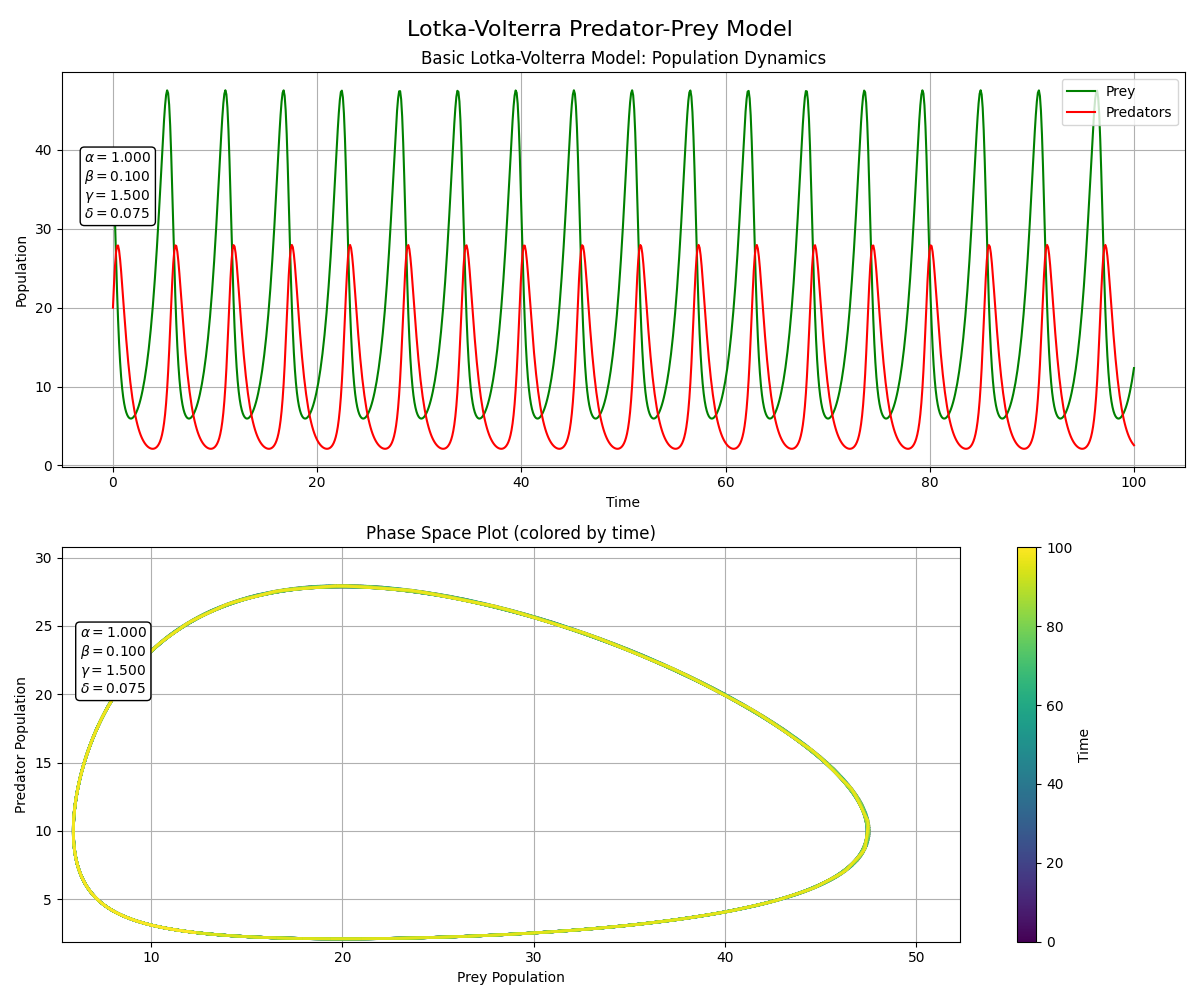
About

Lotka-Volterra predator-prey model simulation, highlighting predator-prey population cycles over time. The mathematical model was independently developed by Lotka (1920) and Volterra (1926).

Features

• Basic Lotka-Volterra model with predator-prey interactions

• Enhanced model with additional ecological factors for realism

• Visualizations of population dynamics and functional responses

• Animated phase space visualization

Lotka-Volterra Model

The Lotka-Volterra model describes predator-prey interactions through a system of non-linear differential equations (Lotka, 1920; Volterra, 1926):

\[ \frac{dx}{dt} = \alpha x - \beta xy \; \; \text{[Prey dynamics]} \] \[ \frac{dy}{dt} = \delta xy - \gamma y \; \; \text{[Predator dynamics]} \]

where:

• \(x\) = Prey population

• \(y\) = Predator population

• \(\alpha\) = Prey growth rate

• \(\beta\) = Predation rate

• \(\gamma\) = Predator death rate

• \(\delta\) = Predator growth rate (due to consuming prey)

Limitations

The basic model has several limitations as discussed by Gurney and Nisbet (1998):

• Unlimited Prey Growth: Assumes exponential prey growth without resource limits.

• Linear Predation Response: Ignores predator satiation and handling time.

• No Time Delays: Immediate population responses, though natural systems show delays.

• Constant Parameters: Ignores seasonal/environmental changes.

• Perfect Cycles: The model predicts ideal cycles, which rarely occur in nature.

A Modified Lotka-Volterra Model

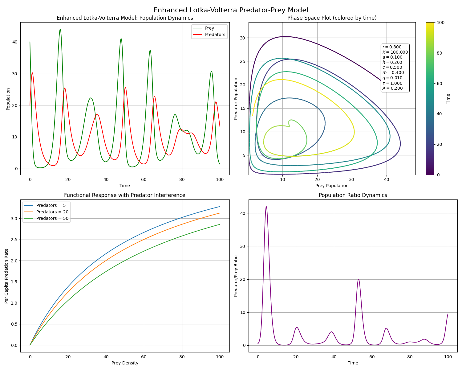
To address some of the limitations of the Lotka-Volterra model, I introduce a modified version of the model that incorporates logistic growth for prey, seasonal variations, time delay, and a Holling Type II functional response with predator interference (Holling, 1959). This model is a combination of the competitive Lotka-Volterra model and the Rosenzweig–MacArthur model (the Lotka-Volterra model with a functional response), along with including a time delay \(\tau\). The modified equations are as follows:

\[ \frac{dx}{dt} = r x \left( 1 - \frac{x}{K} \right) - y S f(x,y) \; \; \text{[Prey dynamics]} \] \[ \frac{dy}{dt}(t) = c y(t) S(t) f\left(x(t-\tau),y(t) \right) - m y(t) \; \; \text{[Predator dynamics]} \]

where:

• \(r\) = Prey growth rate

• \(K\) = Carrying capacity

• \(S(t)\) = Seasonal factor

• \(f(x,y)\) = Functional response

• \(\tau\) = Time delay

• \(m\) = Predator mortality

• \(c\) = Conversion efficiency

The prey growth rate \(r\), is the maximum growth rate of the prey population in the absence of predators; it reflects the reproductive potential of the prey species. The carrying capacity \(K\) is the maximum sustainable population size that the environment can support, taking resource limitations into account. The functional response \(f(x,y)\) describes the relationship between prey density and the rate at which predators consume prey; it captures the non-linear dynamics of predator-prey interactions, accounting for prey availability and predator efficiency. \(\tau\) is the delay for the response of the predator population to changes in the quantity of prey. \(m\), the predator mortality, represents the natural death rate of the predator population; it decreases the predator population over time, regardless of prey population. The conversion efficiency \(c\) is how efficiently predators convert consumed prey into their own biomass; it reflects the energy transfer from prey to predator in the food web. The seasonal factor \(S(t)\) reflects how seasonal variations (like temperature and resource availability) can affect predation and predator growth rates.

In this model, the following seasonal factor was chosen:

\[ S(t) = 1 + A \sin(2 \pi t / 12) \]

and the Beddington–DeAngelis functional response was chosen

\[ f(x,y) = \frac{ax}{1 + a h x + q y} \]

where:

• \(A\) = Amplitude of seasonal variation.

• \(q\) = Interference coefficient

• \(a\) = Attack rate

• \(h\) = Handling time

Limitations

The new model still faces limitations as identified in ecological modeling literature (Gurney & Nisbet, 1998):

• Spatial Homogeneity: Assumes well-mixed populations without spatial structures.

• Age/Size Structure: Ignores differences in age/size within species.

• Species Interactions: Only two species are modeled, while real ecosystems involve more interactions.

• Evolutionary Dynamics: Doesn't account for evolutionary changes over time.

• Environmental Stochasticity: Random environmental factors are excluded.

• Demographic Stochasticity: Birth and death rates are treated deterministically.

• Parameter Sensitivity: The model is sensitive to parameter values that are difficult to measure.

References

[1] Yeakel, J. D., Stiefs, D., Novak, M., & Gross, T. (2011). Generalized modeling of ecological population dynamics. Theoretical Ecology, 4, 179--194. https://doi.org/10.1007/s12080-011-0112-6
[2] Gurney, W. S. C. (1998). Ecological dynamics.
[3] Holling, C. S. (1959). The Components of Predation as Revealed by a Study of Small-Mammal Predation of the European Pine Sawfly. The Canadian Entomologist, 91, 293--320. https://doi.org/10.4039/ent91293-5
[4] Lotka, A. J. (1920). Analytical Note on Certain Rhythmic Relations in Organic Systems. Proceedings of the National Academy of Sciences, 6, 410--415. https://doi.org/10.1073/pnas.6.7.410
[5] VOLTERRA, V. (1926). Fluctuations in the Abundance of a Species considered Mathematically1. Nature, 118, 558--560. https://doi.org/10.1038/118558a0